Clustering¶

Introducción¶

Aprendizaje supervisado¶

• Algoritmo es guiado en el proceso de aprendizaje (se le indica qué debe aprender)
• En algoritmo de regresión lineal, el modelo calcula parámetros que mejor se ajustan a datos conocidos
• ¿Qué ocurre si no contamos con esta información?
  • Respuesta: Algoritmos no supervisados

Aprendizaje no supervisado¶

• No existe información previa sobre qué es lo que debe aprender el algoritmo
• El algoritmo tiene libertad para aprender patrones de interés en los datos

Agrupamiento (Clustering)¶

• Al igual que en clasificación, clustering asigna cada dato a un grupo
• En el caso de clustering, los grupos no son conocidos de antemano

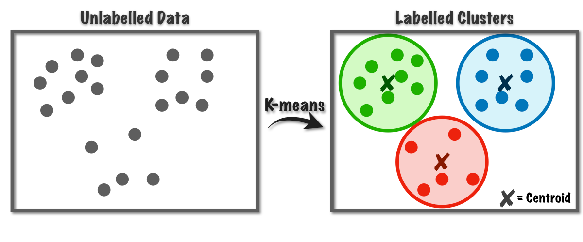
K-Means¶

• K-Means permite agrupar datos a partir de un número especificado de clusters.
• Para K-Means es necesario especificar el número de clusters de antemano. En algunos casos este número sera obvio, pero en otros no.
• Cada clúster se marca inicialmente con un centroide. Este se va actualizando hasta ajustarse a las agrupaciones existentes

In [1]:

from sklearn.datasets import load_iris
import matplotlib.pyplot as plt

iris = load_iris()
X = iris.data[:,2:]
y = iris.target

fig = plt.figure(figsize=(13,4))
ax1 = fig.add_subplot(1,2,1)
ax1.plot(X[y==0,0],X[y==0,1],'yo')
ax1.plot(X[y==1,0],X[y==1,1],'bs')
ax1.plot(X[y==2,0],X[y==2,1],'g^')
ax1.legend(['Iris-Setosa','Iris-Versicolor','Iris-Virginica'])
ax1.set_xlabel('Petal length')
ax1.set_ylabel('Petal width')


ax2 = fig.add_subplot(1,2,2)
ax2.plot(X[:, 0],X[:,1],'k.')
ax2.set_xlabel('Petal length')
ax2.set_ylabel('Petal width')

from sklearn.datasets import load_iris import matplotlib.pyplot as plt iris = load_iris() X = iris.data[:,2:] y = iris.target fig = plt.figure(figsize=(13,4)) ax1 = fig.add_subplot(1,2,1) ax1.plot(X[y==0,0],X[y==0,1],'yo') ax1.plot(X[y==1,0],X[y==1,1],'bs') ax1.plot(X[y==2,0],X[y==2,1],'g^') ax1.legend(['Iris-Setosa','Iris-Versicolor','Iris-Virginica']) ax1.set_xlabel('Petal length') ax1.set_ylabel('Petal width') ax2 = fig.add_subplot(1,2,2) ax2.plot(X[:, 0],X[:,1],'k.') ax2.set_xlabel('Petal length') ax2.set_ylabel('Petal width')

Out[1]:

Text(0, 0.5, 'Petal width')

In [9]:

# Entrenamiento de K-Means
from sklearn.cluster import KMeans

k = 3 # Este es el número de agrupaciones (nuestro supuesto)
kmeans = KMeans(n_clusters=k)
# OJO, no es que nos falte la división en training y test. NO es necesaria en este caso.
kmeans.fit(X)

y_pred = kmeans.predict(X)

# Entrenamiento de K-Means from sklearn.cluster import KMeans k = 3 # Este es el número de agrupaciones (nuestro supuesto) kmeans = KMeans(n_clusters=k) # OJO, no es que nos falte la división en training y test. NO es necesaria en este caso. kmeans.fit(X) y_pred = kmeans.predict(X)

In [10]:

import matplotlib.pyplot as plt

fig = plt.figure(figsize=(13,4))
ax1 = fig.add_subplot(1,2,1)
ax1.plot(X[y==0,0],X[y==0,1],'yo')
ax1.plot(X[y==1,0],X[y==1,1],'bs')
ax1.plot(X[y==2,0],X[y==2,1],'g^')
ax1.legend(['Iris-Setosa','Iris-Versicolor','Iris-Virginica'])
ax1.set_xlabel('Petal length')
ax1.set_ylabel('Petal width')

# Índice de agrupación cambia, pero agrupaciones se mantienen
ax2 = fig.add_subplot(1,2,2)
ax2.plot(X[y_pred==0,0],X[y_pred==0,1],'yo')
ax2.plot(X[y_pred==1,0],X[y_pred==1,1],'g^')
ax2.plot(X[y_pred==2,0],X[y_pred==2,1],'bs')
# ax2.plot(X[y_pred==3,0],X[y_pred==3,1],'k*')
ax2.set_xlabel('Petal length')
ax2.set_ylabel('Petal width')

plt.show()

# Score representa la inercia del modelo (distancia cuadrática media entre cada dato y su centroide)
# Se muestra con valor negativo pues método score de scikit learn debe cumplir con
# "mayor valor, mejor"
print(kmeans.score(X))

import matplotlib.pyplot as plt fig = plt.figure(figsize=(13,4)) ax1 = fig.add_subplot(1,2,1) ax1.plot(X[y==0,0],X[y==0,1],'yo') ax1.plot(X[y==1,0],X[y==1,1],'bs') ax1.plot(X[y==2,0],X[y==2,1],'g^') ax1.legend(['Iris-Setosa','Iris-Versicolor','Iris-Virginica']) ax1.set_xlabel('Petal length') ax1.set_ylabel('Petal width') # Índice de agrupación cambia, pero agrupaciones se mantienen ax2 = fig.add_subplot(1,2,2) ax2.plot(X[y_pred==0,0],X[y_pred==0,1],'yo') ax2.plot(X[y_pred==1,0],X[y_pred==1,1],'g^') ax2.plot(X[y_pred==2,0],X[y_pred==2,1],'bs') # ax2.plot(X[y_pred==3,0],X[y_pred==3,1],'k*') ax2.set_xlabel('Petal length') ax2.set_ylabel('Petal width') plt.show() # Score representa la inercia del modelo (distancia cuadrática media entre cada dato y su centroide) # Se muestra con valor negativo pues método score de scikit learn debe cumplir con # "mayor valor, mejor" print(kmeans.score(X))

-31.37135897435897

Método del codo¶

• En caso de no conocer el número de clusters, una buena aproximación es el método del codo
• Se selecciona como número de clusters a aquel que produce el último decremento importante en la inercia.

In [11]:

score = []
k_clusters = range(1,20) # Este range va de 1 a 20
for k in k_clusters:
    kmeans = KMeans(n_clusters=k)
    kmeans.fit(X)
    score.append(-kmeans.score(X))
    
plt.plot(k_clusters, score,'b.-')

score = [] k_clusters = range(1,20) # Este range va de 1 a 20 for k in k_clusters: kmeans = KMeans(n_clusters=k) kmeans.fit(X) score.append(-kmeans.score(X)) plt.plot(k_clusters, score,'b.-')

Out[11]:

[<matplotlib.lines.Line2D at 0x7f15945fbe80>]

Agrupamiento Jerárquico¶

• Algoritmo que define jerarquía en los datos para generar agrupaciones

• Agrupamiento aglomerativo: A partir de los datos individuales, se agrupan gradualmente hasta formar uno o mútiples grandes grupos. Aproximación bottom up.
• Agrupamiento divisional: A partir de los datos agrupados, se dividen gradualmente hasta formar mútiples grupos pequeños. Aproximación Up bottom

In [17]:

from sklearn.cluster import AgglomerativeClustering

# Escalamiento "puede" mejorar clusterings generados
# # Escalamiento de datos 
# scaler = StandardScaler()
# # Ajustar y transformar datos
# X_scaled = scaler.fit_transform(X)


agg_cluster = AgglomerativeClustering(n_clusters=3)
y_pred = agg_cluster.fit_predict(X)

from sklearn.cluster import AgglomerativeClustering # Escalamiento "puede" mejorar clusterings generados # # Escalamiento de datos # scaler = StandardScaler() # # Ajustar y transformar datos # X_scaled = scaler.fit_transform(X) agg_cluster = AgglomerativeClustering(n_clusters=3) y_pred = agg_cluster.fit_predict(X)

In [13]:

print(y_pred)

print(y_pred)

[1 1 1 1 1 1 1 1 1 1 1 1 1 1 1 1 1 1 1 1 1 1 1 1 1 1 1 1 1 1 1 1 1 1 1 1 1
 1 1 1 1 1 1 1 1 1 1 1 1 1 2 2 0 2 2 2 2 2 2 2 2 2 2 2 2 2 2 2 2 2 0 2 0 2
 2 2 2 0 2 2 2 2 2 0 2 2 2 2 2 2 2 2 2 2 2 2 2 2 2 2 0 0 0 0 0 0 2 0 0 0 0
 0 0 0 0 0 0 0 0 0 0 0 0 0 0 0 0 0 0 0 0 0 0 0 0 0 0 0 0 0 0 0 0 0 0 0 0 0
 0 0]

In [14]:

import matplotlib.pyplot as plt

fig = plt.figure(figsize=(13,4))
ax1 = fig.add_subplot(1,2,1)
ax1.plot(X[y==0,0],X[y==0,1],'yo')
ax1.plot(X[y==1,0],X[y==1,1],'bs')
ax1.plot(X[y==2,0],X[y==2,1],'g^')
ax1.legend(['Iris-Setosa','Iris-Versicolor','Iris-Virginica'])
ax1.set_xlabel('Petal length')
ax1.set_ylabel('Petal width')

# Índice de agrupación cambia, pero agrupaciones se mantienen
ax2 = fig.add_subplot(1,2,2)
ax2.plot(X[y_pred==0,0],X[y_pred==0,1],'g^')
ax2.plot(X[y_pred==1,0],X[y_pred==1,1],'yo')
ax2.plot(X[y_pred==2,0],X[y_pred==2,1],'bs')
ax2.set_xlabel('Petal length')
ax2.set_ylabel('Petal width')

plt.show()

import matplotlib.pyplot as plt fig = plt.figure(figsize=(13,4)) ax1 = fig.add_subplot(1,2,1) ax1.plot(X[y==0,0],X[y==0,1],'yo') ax1.plot(X[y==1,0],X[y==1,1],'bs') ax1.plot(X[y==2,0],X[y==2,1],'g^') ax1.legend(['Iris-Setosa','Iris-Versicolor','Iris-Virginica']) ax1.set_xlabel('Petal length') ax1.set_ylabel('Petal width') # Índice de agrupación cambia, pero agrupaciones se mantienen ax2 = fig.add_subplot(1,2,2) ax2.plot(X[y_pred==0,0],X[y_pred==0,1],'g^') ax2.plot(X[y_pred==1,0],X[y_pred==1,1],'yo') ax2.plot(X[y_pred==2,0],X[y_pred==2,1],'bs') ax2.set_xlabel('Petal length') ax2.set_ylabel('Petal width') plt.show()

In [15]:

# Dendograma (gráfico de conexiones de agrupamientos)
import scipy.cluster.hierarchy as sch
from sklearn.preprocessing import StandardScaler

plt.figure(figsize = (15, 6))
sch.dendrogram(sch.linkage(X, method = 'ward'))
plt.xlabel('Data Points');

# Dendograma (gráfico de conexiones de agrupamientos) import scipy.cluster.hierarchy as sch from sklearn.preprocessing import StandardScaler plt.figure(figsize = (15, 6)) sch.dendrogram(sch.linkage(X, method = 'ward')) plt.xlabel('Data Points');

DBSCAN¶

• Density-based spatial clustering of applications with noise
• Algoritmo capaz de identificar clúster de agrupación en base a la "densidad" de los datos.
• Paso a paso:
  • Por cada instancia, se cuentan cuántas instancias están dentro de una distancia $\epsilon$ (vecindario $\epsilon$)
  • Si una instancia tienen al menos min_samples instancias en su vecindario, es considerada una instancia core.
  • Todas las instancias en el vecindario de una instancia core pertenecen al mismo clúster (incluídas otras instancias core).
  • Cualquier instancia que no sea una instancia core o no pertenezca a un vecindario, es considerada anomalía.

In [ ]:

from sklearn.cluster import DBSCAN

dbscan = DBSCAN(eps=0.2, min_samples=4)
y_pred = dbscan.fit_predict(X)
print(y_pred)

from sklearn.cluster import DBSCAN dbscan = DBSCAN(eps=0.2, min_samples=4) y_pred = dbscan.fit_predict(X) print(y_pred)

In [ ]:

import matplotlib.pyplot as plt

fig = plt.figure(figsize=(13,4))
ax1 = fig.add_subplot(1,2,1)
ax1.plot(X[y==0,0],X[y==0,1],'yo')
ax1.plot(X[y==1,0],X[y==1,1],'bs')
ax1.plot(X[y==2,0],X[y==2,1],'g^')
ax1.legend(['Iris-Setosa','Iris-Versicolor','Iris-Virginica'])
ax1.set_xlabel('Petal length')
ax1.set_ylabel('Petal width')

# Índice de agrupación cambia, pero agrupaciones se mantienen
ax2 = fig.add_subplot(1,2,2)
ax2.plot(X[y_pred==-1,0],X[y_pred==-1,1],'r*') # Anomalías
ax2.plot(X[y_pred==0,0],X[y_pred==0,1],'yo')
ax2.plot(X[y_pred==1,0],X[y_pred==1,1],'bs')
ax2.plot(X[y_pred==2,0],X[y_pred==2,1],'g^')
ax2.legend(['Anomalías', 'Iris-Setosa','Iris-Versicolor','Iris-Virginica'])
ax2.set_xlabel('Petal length')
ax2.set_ylabel('Petal width')

plt.show()

import matplotlib.pyplot as plt fig = plt.figure(figsize=(13,4)) ax1 = fig.add_subplot(1,2,1) ax1.plot(X[y==0,0],X[y==0,1],'yo') ax1.plot(X[y==1,0],X[y==1,1],'bs') ax1.plot(X[y==2,0],X[y==2,1],'g^') ax1.legend(['Iris-Setosa','Iris-Versicolor','Iris-Virginica']) ax1.set_xlabel('Petal length') ax1.set_ylabel('Petal width') # Índice de agrupación cambia, pero agrupaciones se mantienen ax2 = fig.add_subplot(1,2,2) ax2.plot(X[y_pred==-1,0],X[y_pred==-1,1],'r*') # Anomalías ax2.plot(X[y_pred==0,0],X[y_pred==0,1],'yo') ax2.plot(X[y_pred==1,0],X[y_pred==1,1],'bs') ax2.plot(X[y_pred==2,0],X[y_pred==2,1],'g^') ax2.legend(['Anomalías', 'Iris-Setosa','Iris-Versicolor','Iris-Virginica']) ax2.set_xlabel('Petal length') ax2.set_ylabel('Petal width') plt.show()

Actividad 8¶

Scikit Learn no solo provee algunos datasets populares. También incluye toy datasets, los cuales son datasets para comprobar las particularidades de distintos modelos.

• Estudie el toy dataset Make Moons disponible en scikit learn aquí
• Genere un dataset con 1000 muestras y ruido (noise) $0.05$.
• Utilice los distintos algoritmos de clustering para identificar agrupaciones de datos. Utilice matplotlib para mostrar gráficamente cuál de ellos se ajusta mejor.