Writing Efficient Queries
Introduction
Sometimes it doesn't matter whether your query is efficient or not. For example, you might write a query you expect to run only once, and it might be working on a small dataset. In this case, anything that gives you the answer you need will do.
But what about queries that will be run many times, like a query that feeds data to a website? Those need to be efficient so you don't leave users waiting for your website to load.
Or what about queries on huge datasets? These can be slow and cost a business a lot of money if they are written poorly.
Most database systems have a query optimizer that attempts to interpret/execute your query in the most effective way possible. But several strategies can still yield huge savings in many cases.
Some useful functions
We will use two functions to compare the efficiency of different queries:
show_amount_of_data_scanned()shows the amount of data the query uses.show_time_to_run()prints how long it takes for the query to execute.
from google.cloud import bigquery
from time import time

client = bigquery.Client()

def show_amount_of_data_scanned(query):
    # dry_run lets us see how much data the query uses without running it
    dry_run_config = bigquery.QueryJobConfig(dry_run=True)
    query_job = client.query(query, job_config=dry_run_config)
    print('Data processed: {} GB'.format(round(query_job.total_bytes_processed / 10**9, 3)))

def show_time_to_run(query):
    time_config = bigquery.QueryJobConfig(use_query_cache=False)
    start = time()
    query_result = client.query(query, job_config=time_config).result()
    end = time()
    print('Time to run: {} seconds'.format(round(end-start, 3)))
Using Kaggle's public dataset BigQuery integration.
Strategies
1) Only select the columns you want.
It is tempting to start queries with SELECT * FROM .... It's convenient because you don't need to think about which columns you need. But it can be very inefficient.
This is especially important if there are text fields that you don't need, because text fields tend to be larger than other fields.
star_query = "SELECT * FROM `bigquery-public-data.github_repos.contents`"
show_amount_of_data_scanned(star_query)

basic_query = "SELECT size, binary FROM `bigquery-public-data.github_repos.contents`"
show_amount_of_data_scanned(basic_query)
Data processed: 2623.284 GB
Data processed: 2.466 GB
In this case, we see a 1000X reduction in data being scanned to complete the query, because the raw data contained a text field that was 1000X larger than the fields we might need.
2) Read less data.
Both queries below calculate the average duration (in seconds) of one-way bike trips in the city of San Francisco.
more_data_query = """
                  SELECT MIN(start_station_name) AS start_station_name,
                      MIN(end_station_name) AS end_station_name,
                      AVG(duration_sec) AS avg_duration_sec
                  FROM `bigquery-public-data.san_francisco.bikeshare_trips`
                  WHERE start_station_id != end_station_id
                  GROUP BY start_station_id, end_station_id
                  LIMIT 10
                  """
show_amount_of_data_scanned(more_data_query)

less_data_query = """
                  SELECT start_station_name,
                      end_station_name,
                      AVG(duration_sec) AS avg_duration_sec
                  FROM `bigquery-public-data.san_francisco.bikeshare_trips`
                  WHERE start_station_name != end_station_name
                  GROUP BY start_station_name, end_station_name
                  LIMIT 10
                  """
show_amount_of_data_scanned(less_data_query)
Data processed: 0.076 GB
Data processed: 0.06 GB
Since there is a 1:1 relationship between the station ID and the station name, we don't need to use the start_station_id and end_station_id columns in the query. By using only the columns with the station IDs, we scan less data.
3) Avoid N:N JOINs.
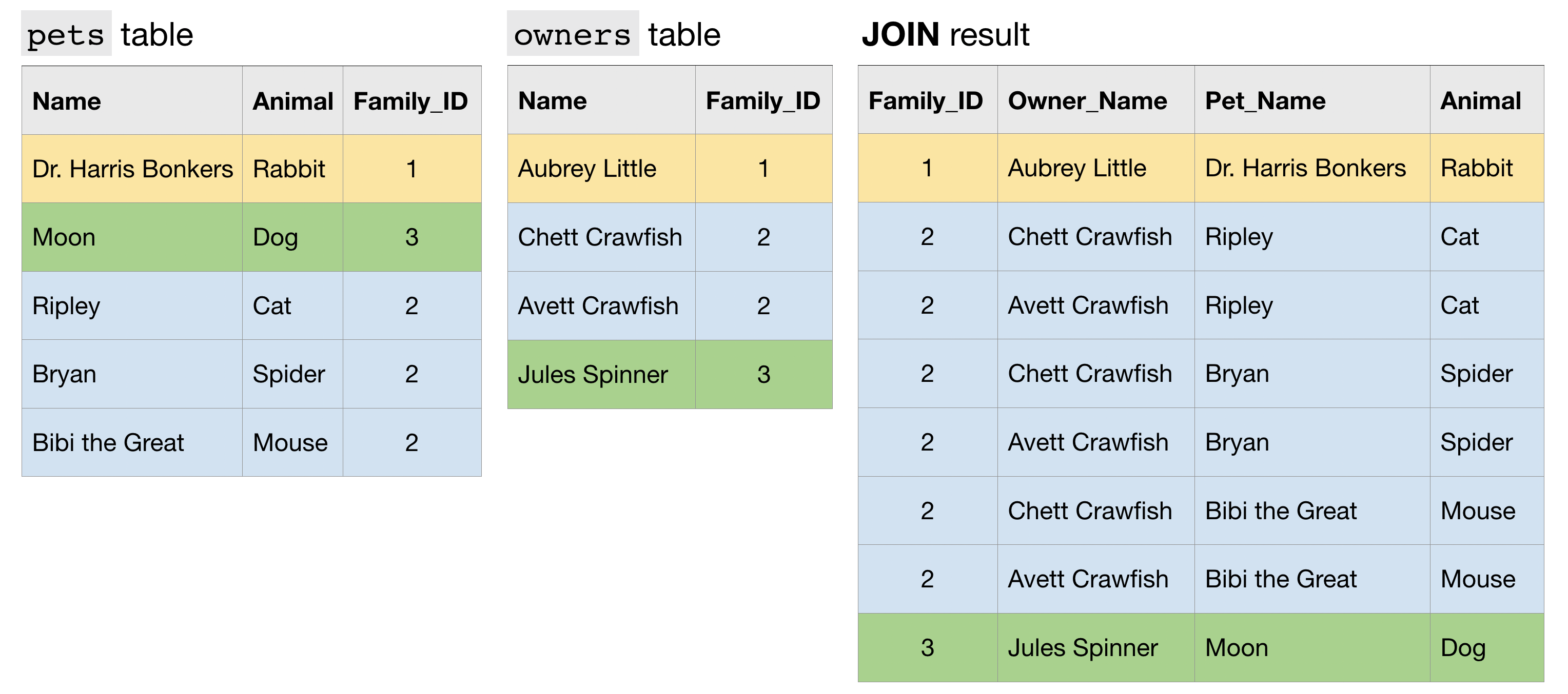
Most of the JOINs that you have executed in this course have been 1:1 JOINs. In this case, each row in each table has at most one match in the other table.

Another type of JOIN is an N:1 JOIN. Here, each row in one table matches potentially many rows in the other table.

Finally, an N:N JOIN is one where a group of rows in one table can match a group of rows in the other table. Note that in general, all other things equal, this type of JOIN produces a table with many more rows than either of the two (original) tables that are being JOINed.

Now we'll work with an example from a real dataset. Both examples below count the number of distinct committers and the number of files in several GitHub repositories.
big_join_query = """
                 SELECT repo,
                     COUNT(DISTINCT c.committer.name) as num_committers,
                     COUNT(DISTINCT f.id) AS num_files
                 FROM `bigquery-public-data.github_repos.commits` AS c,
                     UNNEST(c.repo_name) AS repo
                 INNER JOIN `bigquery-public-data.github_repos.files` AS f
                     ON f.repo_name = repo
                 WHERE f.repo_name IN ( 'tensorflow/tensorflow', 'facebook/react', 'twbs/bootstrap', 'apple/swift', 'Microsoft/vscode', 'torvalds/linux')
                 GROUP BY repo
                 ORDER BY repo
                 """
show_time_to_run(big_join_query)

small_join_query = """
                   WITH commits AS
                   (
                   SELECT COUNT(DISTINCT committer.name) AS num_committers, repo
                   FROM `bigquery-public-data.github_repos.commits`,
                       UNNEST(repo_name) as repo
                   WHERE repo IN ( 'tensorflow/tensorflow', 'facebook/react', 'twbs/bootstrap', 'apple/swift', 'Microsoft/vscode', 'torvalds/linux')
                   GROUP BY repo
                   ),
                   files AS
                   (
                   SELECT COUNT(DISTINCT id) AS num_files, repo_name as repo
                   FROM `bigquery-public-data.github_repos.files`
                   WHERE repo_name IN ( 'tensorflow/tensorflow', 'facebook/react', 'twbs/bootstrap', 'apple/swift', 'Microsoft/vscode', 'torvalds/linux')
                   GROUP BY repo
                   )
                   SELECT commits.repo, commits.num_committers, files.num_files
                   FROM commits
                   INNER JOIN files
                       ON commits.repo = files.repo
                   ORDER BY repo
                   """

show_time_to_run(small_join_query)
Time to run: 11.926 seconds
Time to run: 4.293 seconds
The first query has a large N:N JOIN. By rewriting the query to decrease the size of the JOIN, we see it runs much faster.
Learn more
These strategies and many more are discussed in this thorough guide to Google BigQuery. If you'd like to learn more about how to write more efficient queries (or deepen your knowledge of all things BigQuery), you're encouraged to check it out!
Your turn
Leverage what you've learned to improve the design of several queries.
Have questions or comments? Visit the course discussion forum to chat with other learners.
