Pandas II¶

"Pandas es a los datos tabulares lo que NumPy es a los arreglos numéricos: la herramienta que hace que todo lo demás tenga sentido."

Introducción¶

En Pandas I aprendiste a cargar, explorar, filtrar y limpiar datos. En esta clase vas un paso más allá: agregar, combinar y reshapear DataFrames, y terminas con una primera mirada a Seaborn para visualizar los resultados.

En este módulo aprenderás a:

• Agrupar y resumir datos con groupby
• Combinar tablas con concat y merge
• Cambiar la forma de una tabla con pivot y melt
• Visualizar datos estadísticos con Seaborn básico

In [36]:

import pandas as pd
import numpy as np
import seaborn as sns
import matplotlib.pyplot as plt

# Dataset NBA Players
path = "https://raw.githubusercontent.com/fralfaro/MAT281/main/docs/lectures/data_manipulation/data/player_info.csv"
df = pd.read_csv(path).dropna()
df["decade"] = df["year_start"].apply(lambda x: "2000s" if x >= 2000 else "1900s")
df.head()

import pandas as pd import numpy as np import seaborn as sns import matplotlib.pyplot as plt # Dataset NBA Players path = "https://raw.githubusercontent.com/fralfaro/MAT281/main/docs/lectures/data_manipulation/data/player_info.csv" df = pd.read_csv(path).dropna() df["decade"] = df["year_start"].apply(lambda x: "2000s" if x >= 2000 else "1900s") df.head()

Out[36]:

	name	year_start	year_end	position	height	weight	birth_date	college	decade
2	Zaid Abdul-Aziz	1969	1978	C-F	6-9	235.0	April 7, 1946	Iowa State University	1900s
3	Kareem Abdul-Jabbar	1970	1989	C	7-2	225.0	April 16, 1947	University of California, Los Angeles	1900s
4	Mahmoud Abdul-Rauf	1991	2001	G	6-1	162.0	March 9, 1969	Louisiana State University	1900s
5	Tariq Abdul-Wahad	1998	2003	F	6-6	223.0	November 3, 1974	San Jose State University	1900s
6	Shareef Abdur-Rahim	1997	2008	F	6-9	225.0	December 11, 1976	University of California	1900s

Groupby¶

Groupby divide el DataFrame en grupos, aplica una función a cada grupo, y combina los resultados. Es el equivalente a un GROUP BY en SQL.

dividir → aplicar → combinar

Agrupar por una columna¶

In [37]:

# Peso promedio por posición
df.groupby("position")["weight"].mean()

# Peso promedio por posición df.groupby("position")["weight"].mean()

Out[37]:

	weight
position
C	242.219212
C-F	228.256158
F	217.985857
F-C	222.871866
F-G	202.604878
G	186.828115
G-F	197.017857

dtype: float64

Agrupar por varias columnas¶

In [38]:

# Peso promedio por década y posición
df.groupby(["decade", "position"])["weight"].mean().head(10)

# Peso promedio por década y posición df.groupby(["decade", "position"])["weight"].mean().head(10)

Out[38]:

		weight
decade	position
1900s	C	237.453642
	C-F	224.871345
	F	212.582933
	F-C	217.908475
	F-G	200.594444
	G	182.689150
	G-F	192.789062
2000s	C	256.057692
	C-F	246.343750
	F	230.135135

dtype: float64

Múltiples funciones¶

In [39]:

# Estadísticas de peso y año de inicio por grupo
df.groupby(["decade", "position"]).agg({
    "weight":     ["min", "max", "mean"],
    "year_start": ["min", "max"]
}).head()

# Estadísticas de peso y año de inicio por grupo df.groupby(["decade", "position"]).agg({ "weight": ["min", "max", "mean"], "year_start": ["min", "max"] }).head()

Out[39]:

		weight			year_start
		min	max	mean	min	max
decade	position
1900s	C	190.0	330.0	237.453642	1947	1999
	C-F	185.0	270.0	224.871345	1947	1998
	F	165.0	284.0	212.582933	1947	1999
	F-C	180.0	290.0	217.908475	1947	1999
	F-G	165.0	245.0	200.594444	1947	1999

Función personalizada¶

In [40]:

def promedio_armonico(serie):
    return len(serie) / sum(1 / x for x in serie)

df.groupby(["decade", "position"])["weight"].apply(promedio_armonico).head()

def promedio_armonico(serie): return len(serie) / sum(1 / x for x in serie) df.groupby(["decade", "position"])["weight"].apply(promedio_armonico).head()

Out[40]:

		weight
decade	position
1900s	C	235.811208
	C-F	223.766067
	F	211.205181
	F-C	216.785001
	F-G	199.669744

dtype: float64

Transform¶

El transform es útil para comparar cada registro contra su grupo, por ejemplo:

• df["peso_vs_media"] = df["weight"] - df["mean_weight_group"]

In [41]:

# Agrega la media del grupo como nueva columna (mantiene el índice original)
df["mean_weight_group"] = df.groupby(["decade", "position"])["weight"].transform("mean")
df[["name", "position", "decade", "weight", "mean_weight_group"]].head()

# Agrega la media del grupo como nueva columna (mantiene el índice original) df["mean_weight_group"] = df.groupby(["decade", "position"])["weight"].transform("mean") df[["name", "position", "decade", "weight", "mean_weight_group"]].head()

Out[41]:

	name	position	decade	weight	mean_weight_group
2	Zaid Abdul-Aziz	C-F	1900s	235.0	224.871345
3	Kareem Abdul-Jabbar	C	1900s	225.0	237.453642
4	Mahmoud Abdul-Rauf	G	1900s	162.0	182.689150
5	Tariq Abdul-Wahad	F	1900s	223.0	212.582933
6	Shareef Abdur-Rahim	F	1900s	225.0	212.582933

Filter¶

In [42]:

# Solo posiciones cuyo peso promedio supera 220 lbs
df.groupby("position").filter(lambda x: x["weight"].mean() > 220).head()

# Solo posiciones cuyo peso promedio supera 220 lbs df.groupby("position").filter(lambda x: x["weight"].mean() > 220).head()

Out[42]:

	name	year_start	year_end	position	height	weight	birth_date	college	decade	mean_weight_group
2	Zaid Abdul-Aziz	1969	1978	C-F	6-9	235.0	April 7, 1946	Iowa State University	1900s	224.871345
3	Kareem Abdul-Jabbar	1970	1989	C	7-2	225.0	April 16, 1947	University of California, Los Angeles	1900s	237.453642
13	Mark Acres	1988	1993	F-C	6-11	220.0	November 15, 1962	Oral Roberts University	1900s	217.908475
16	Alvan Adams	1976	1988	C-F	6-9	210.0	July 19, 1954	University of Oklahoma	1900s	224.871345
22	Steven Adams	2014	2018	C	7-0	255.0	July 20, 1993	University of Pittsburgh	2000s	256.057692

Concat¶

El pd.concat() apila DataFrames.

In [43]:

df_antes_2000  = df.loc[df["year_start"] < 2000]
df_desde_2000  = df.loc[df["year_start"] >= 2000]

# Mismas columnas → apila filas
result = pd.concat([df_antes_2000, df_desde_2000])
print(result.shape)   # misma cantidad de columnas

df_antes_2000 = df.loc[df["year_start"] < 2000] df_desde_2000 = df.loc[df["year_start"] >= 2000] # Mismas columnas → apila filas result = pd.concat([df_antes_2000, df_desde_2000]) print(result.shape) # misma cantidad de columnas

(4212, 10)

Si las columnas no coinciden exactamente, pandas rellena con NaN:

In [44]:

df_desde_2000_mod = df_desde_2000.rename(columns={"birth_date": "birth"})
result = pd.concat([df_antes_2000, df_desde_2000_mod])
result.columns   # aparecen birth_date Y birth como columnas separadas

df_desde_2000_mod = df_desde_2000.rename(columns={"birth_date": "birth"}) result = pd.concat([df_antes_2000, df_desde_2000_mod]) result.columns # aparecen birth_date Y birth como columnas separadas

Out[44]:

Index(['name', 'year_start', 'year_end', 'position', 'height', 'weight',
       'birth_date', 'college', 'decade', 'mean_weight_group', 'birth'],
      dtype='object')

Usa ignore_index=True si quieres resetear el índice después de concatenar: pd.concat([df1, df2], ignore_index=True)

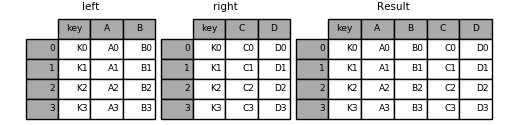
Merge¶

El pd.merge() combina dos DataFrames por una o más columnas comunes. Es el equivalente a un JOIN en SQL.

In [45]:

df_info    = df[["name", "year_start", "year_end", "position"]]
df_fisico  = df[["name", "height", "weight", "college"]]

# Inner join por nombre
result = pd.merge(df_info, df_fisico, on="name")
result.head()

df_info = df[["name", "year_start", "year_end", "position"]] df_fisico = df[["name", "height", "weight", "college"]] # Inner join por nombre result = pd.merge(df_info, df_fisico, on="name") result.head()

Out[45]:

	name	year_start	year_end	position	height	weight	college
0	Zaid Abdul-Aziz	1969	1978	C-F	6-9	235.0	Iowa State University
1	Kareem Abdul-Jabbar	1970	1989	C	7-2	225.0	University of California, Los Angeles
2	Mahmoud Abdul-Rauf	1991	2001	G	6-1	162.0	Louisiana State University
3	Tariq Abdul-Wahad	1998	2003	F	6-6	223.0	San Jose State University
4	Shareef Abdur-Rahim	1997	2008	F	6-9	225.0	University of California

Por un columna

Por Varias columnas

Tipos de merge

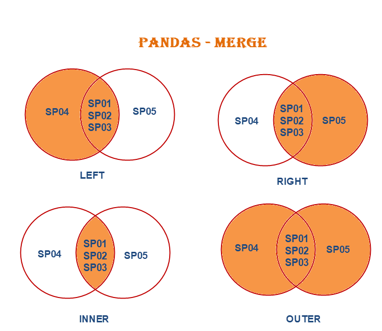
La opción how especificica el tipo de cruce que se realizará.

Tipo	Descripción	SQL equivalente
inner	Solo filas con coincidencia en ambas tablas	INNER JOIN
left	Todas las filas de la izquierda	LEFT JOIN
right	Todas las filas de la derecha	RIGHT JOIN
outer	Unión de ambas tablas	FULL OUTER JOIN

In [46]:

print("inner join — solo coincidencias en ambas tablas")
display(pd.merge(df_info, df_fisico, on="name", how="inner").head())

print("left join — todas las filas de df_info")
display(pd.merge(df_info, df_fisico, on="name", how="left").head())

print("outer join — unión completa de ambas tablas")
display(pd.merge(df_info, df_fisico, on="name", how="outer").head())

print("inner join — solo coincidencias en ambas tablas") display(pd.merge(df_info, df_fisico, on="name", how="inner").head()) print("left join — todas las filas de df_info") display(pd.merge(df_info, df_fisico, on="name", how="left").head()) print("outer join — unión completa de ambas tablas") display(pd.merge(df_info, df_fisico, on="name", how="outer").head())

inner join — solo coincidencias en ambas tablas

	name	year_start	year_end	position	height	weight	college
0	Zaid Abdul-Aziz	1969	1978	C-F	6-9	235.0	Iowa State University
1	Kareem Abdul-Jabbar	1970	1989	C	7-2	225.0	University of California, Los Angeles
2	Mahmoud Abdul-Rauf	1991	2001	G	6-1	162.0	Louisiana State University
3	Tariq Abdul-Wahad	1998	2003	F	6-6	223.0	San Jose State University
4	Shareef Abdur-Rahim	1997	2008	F	6-9	225.0	University of California

left join — todas las filas de df_info

	name	year_start	year_end	position	height	weight	college
0	Zaid Abdul-Aziz	1969	1978	C-F	6-9	235.0	Iowa State University
1	Kareem Abdul-Jabbar	1970	1989	C	7-2	225.0	University of California, Los Angeles
2	Mahmoud Abdul-Rauf	1991	2001	G	6-1	162.0	Louisiana State University
3	Tariq Abdul-Wahad	1998	2003	F	6-6	223.0	San Jose State University
4	Shareef Abdur-Rahim	1997	2008	F	6-9	225.0	University of California

outer join — unión completa de ambas tablas

	name	year_start	year_end	position	height	weight	college
0	A.C. Green	1986	2001	F-C	6-9	220.0	Oregon State University
1	A.J. Bramlett	2000	2000	C	6-10	227.0	University of Arizona
2	A.J. English	1991	1992	G	6-3	175.0	Virginia Union University
3	A.J. Guyton	2001	2003	G	6-1	180.0	Indiana University
4	A.J. Hammons	2017	2017	C	7-0	260.0	Purdue University

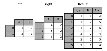
Columnas duplicadas

Cuando ambas tablas tienen una columna con el mismo nombre que no es la clave, pandas la renombra automáticamente con sufijos _x e _y:

In [47]:

df_a = df[["name", "year_start", "year_end", "position"]]
df_b = df[["name", "year_start", "year_end", "height"]]

# year_end aparece en ambas pero no es la clave → year_end_x, year_end_y
pd.merge(df_a, df_b, on=["name", "year_start"]).head()

df_a = df[["name", "year_start", "year_end", "position"]] df_b = df[["name", "year_start", "year_end", "height"]] # year_end aparece en ambas pero no es la clave → year_end_x, year_end_y pd.merge(df_a, df_b, on=["name", "year_start"]).head()

Out[47]:

	name	year_start	year_end_x	position	year_end_y	height
0	Zaid Abdul-Aziz	1969	1978	C-F	1978	6-9
1	Kareem Abdul-Jabbar	1970	1989	C	1989	7-2
2	Mahmoud Abdul-Rauf	1991	2001	G	2001	6-1
3	Tariq Abdul-Wahad	1998	2003	F	2003	6-6
4	Shareef Abdur-Rahim	1997	2008	F	2008	6-9

Formatos wide y long¶

Los datos tabulares pueden presentarse en dos formatos:

Formato	Descripción	Cuándo usarlo
Wide	Cada variable tiene su propia columna	Análisis, ML
Long	Una columna de variable + una de valor	Visualización, groupby

long a wide: pivot

In [48]:

# Peso promedio por década (filas) y posición (columnas)
pivot = df.pivot_table(
    index="decade",
    columns="position",
    values="weight",
    aggfunc="mean"
)
pivot

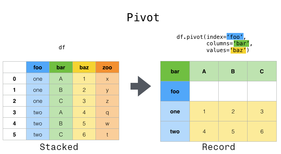
# Peso promedio por década (filas) y posición (columnas) pivot = df.pivot_table( index="decade", columns="position", values="weight", aggfunc="mean" ) pivot

Out[48]:

position	C	C-F	F	F-C	F-G	G	G-F
decade
1900s	237.453642	224.871345	212.582933	217.908475	200.594444	182.689150	192.789062
2000s	256.057692	246.343750	230.135135	245.750000	217.080000	195.686192	210.550000

In [50]:

# pivot: simple
agrupado = df.groupby(['decade','position'])['weight'].mean().reset_index()
pivot_df = agrupado.pivot(index='decade', columns='position', values='weight')
pivot_df.head(10)

# pivot: simple agrupado = df.groupby(['decade','position'])['weight'].mean().reset_index() pivot_df = agrupado.pivot(index='decade', columns='position', values='weight') pivot_df.head(10)

Out[50]:

position	C	C-F	F	F-C	F-G	G	G-F
decade
1900s	237.453642	224.871345	212.582933	217.908475	200.594444	182.689150	192.789062
2000s	256.057692	246.343750	230.135135	245.750000	217.080000	195.686192	210.550000

In [ ]:

# Pivot con múltiples índices
pivot_multi = df.pivot_table(
    index=["decade", "height"],
    columns="position",
    values="weight",
    aggfunc="mean"
).fillna(0)
pivot_multi.head()

# Pivot con múltiples índices pivot_multi = df.pivot_table( index=["decade", "height"], columns="position", values="weight", aggfunc="mean" ).fillna(0) pivot_multi.head()

Out[ ]:

	position	C	C-F	F	F-C	F-G	G	G-F
decade	height
1900s	5-10	0.0	0.0	0.0	0.0	0.0	167.914286	163.333333
	5-11	0.0	0.0	0.0	0.0	175.0	171.666667	171.666667
	5-3	0.0	0.0	0.0	0.0	0.0	136.000000	0.000000
	5-5	0.0	0.0	0.0	0.0	0.0	135.000000	0.000000
	5-6	0.0	0.0	0.0	0.0	0.0	149.000000	0.000000

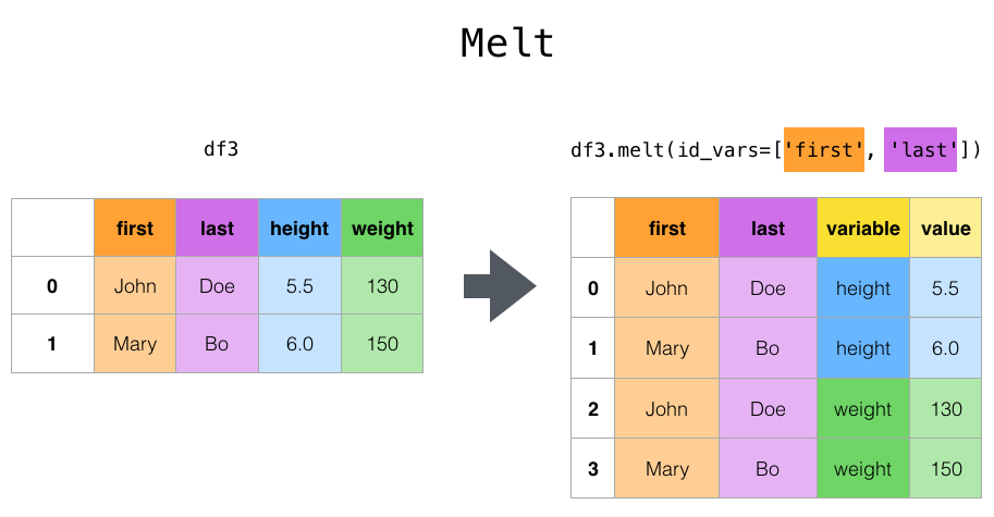
Wide → Long: melt

In [ ]:

# Tenemos tabla wide
df_wide = df.pivot_table(
    index=["name", "year_start", "year_end"],
    columns="position",
    values="weight",
    aggfunc="mean"
).fillna(0).reset_index()
df_wide.columns.name = None

# Volver a long
df_long = df_wide.melt(
    id_vars=["name", "year_start", "year_end"],
    var_name="position",
    value_name="weight"
)
df_long.head()

# Tenemos tabla wide df_wide = df.pivot_table( index=["name", "year_start", "year_end"], columns="position", values="weight", aggfunc="mean" ).fillna(0).reset_index() df_wide.columns.name = None # Volver a long df_long = df_wide.melt( id_vars=["name", "year_start", "year_end"], var_name="position", value_name="weight" ) df_long.head()

Out[ ]:

	name	year_start	year_end	position	weight
0	A.C. Green	1986	2001	C	0.0
1	A.J. Bramlett	2000	2000	C	227.0
2	A.J. English	1991	1992	C	0.0
3	A.J. Guyton	2001	2003	C	0.0
4	A.J. Hammons	2017	2017	C	260.0

Referencias¶

1. Pandas Groupby
2. Pandas Merging
3. Pandas Reshaping